Project 2: Fun with Filters and Frequencies!

Student Name: Kelvin Huang

Part 1: Fun with Filters

Part 1.1: Finite Difference Operator

In this part, we apply the finite difference operator using the humble finite difference as our filter in the x and y directions. This method is essential for calculating image gradients, which help us detect edges and changes in intensity. For edge detection, a threshold of 25 is used.

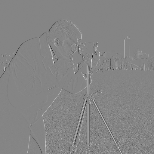
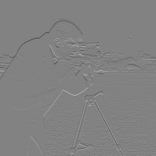
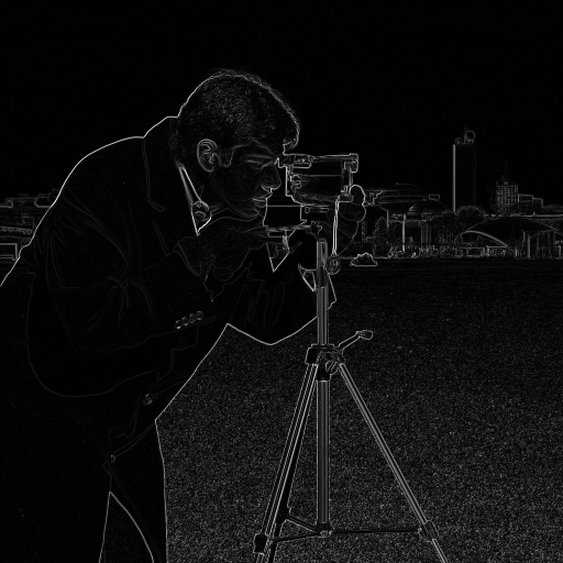
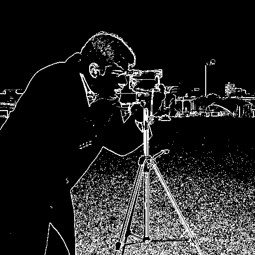
The gradient magnitude represents the strength of the gradient at each pixel and is essential for detecting edges in an image. It is computed by combining the gradients in the x and y directions. After calculating the partial derivatives \( D_x \) and \( D_y \) using the finite difference operators, the gradient magnitude at each pixel is given by the formula:

$$ \text{Gradient Magnitude} = \sqrt{(D_x)^2 + (D_y)^2} $$ This magnitude provides a scalar value representing how much the intensity is changing at a particular point, with higher values corresponding to sharper transitions (edges). By applying a threshold to the gradient magnitude, we can create a binarized edge image that highlights the most prominent edges while reducing noise.

Part 1.2: Derivative of Gaussian (DoG) Filter

In this part, we apply a Gaussian smoothing filter before taking the gradient to reduce noise and improve the robustness of edge detection.

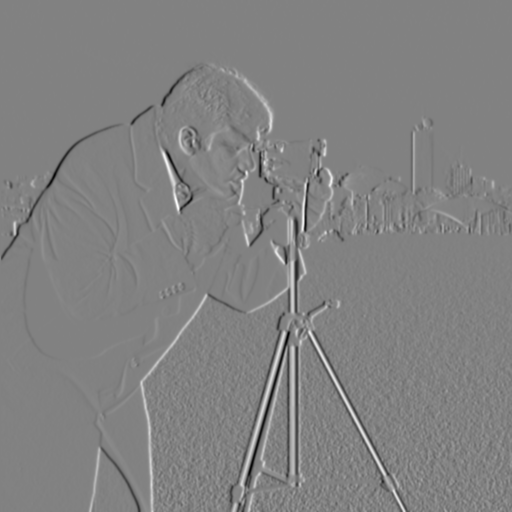
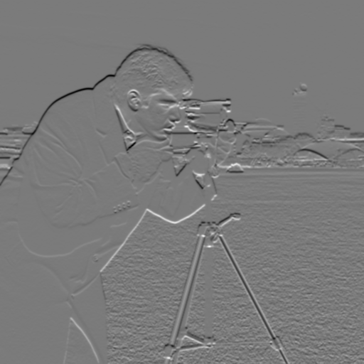
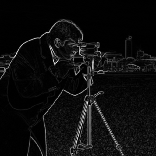
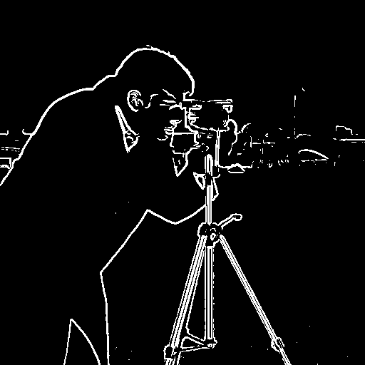
Differences I see: These images appear smoother with reduced noise, while the edges are cleaner and more pronounced. Note: I use a lower threshold here compare to the previous section.

Single Convolution with DoG Filters

Instead of applying two separate operations (smoothing and then calculating gradients), we can use a single convolution with Derivative of Gaussian filters. Here, we create filters by convolving the Gaussian with \(D_x\) and \(D_y\) to compute the gradients directly. Below are the DoG filters and the corresponding gradient and edge images.

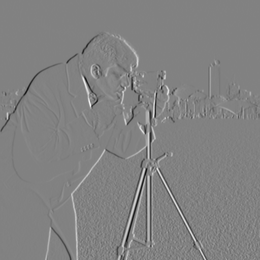
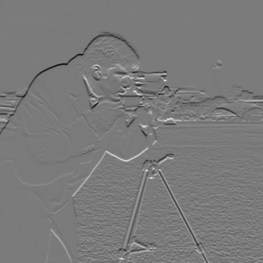
We can see that the result of DoG is same as the method above. Clear and smooth.

Part 2: Fun with Frequencies!

Part 2.1: Image "Sharpening"

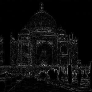
Taj Mahal

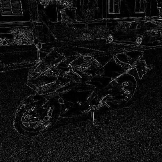
Motorcycle

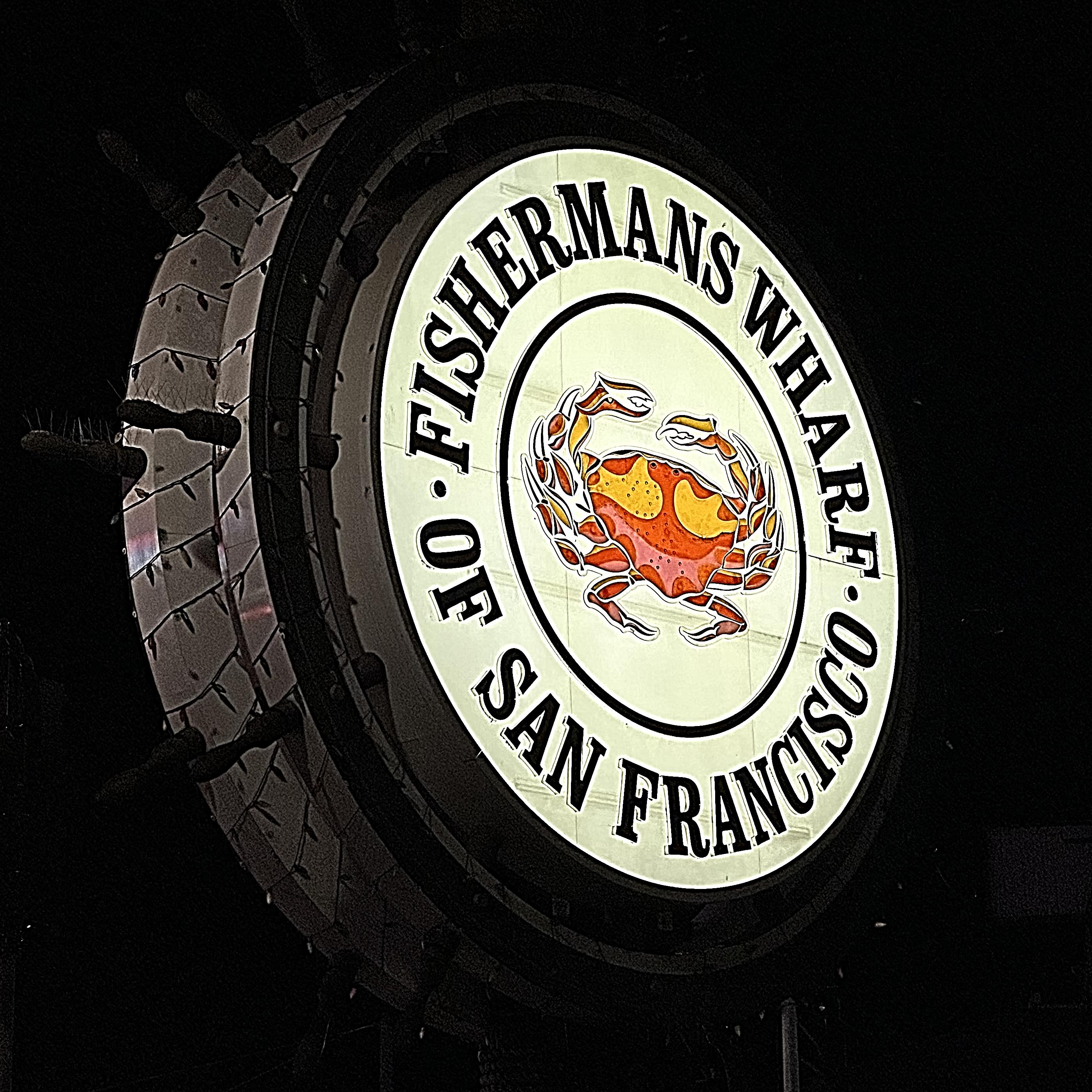
Sharpened After Blurred: Fishermans

Sharpened After Blurred: My Friend Harry on a Kayak

The blurred and sharpened image, in contrast to the original, shows more noise and visual artifacts. Although the edges become sharper and more defined, there’s a noticeable reduction in the clarity of fine details. Many of the intricate elements from the original are either blurred or entirely lost. The sharpening process enhances edge contrast but also introduces unwanted noise, giving the image a more artificial appearance and compromising its overall quality.

Part 2.2: Hybrid Images

Derek and Nutmeg

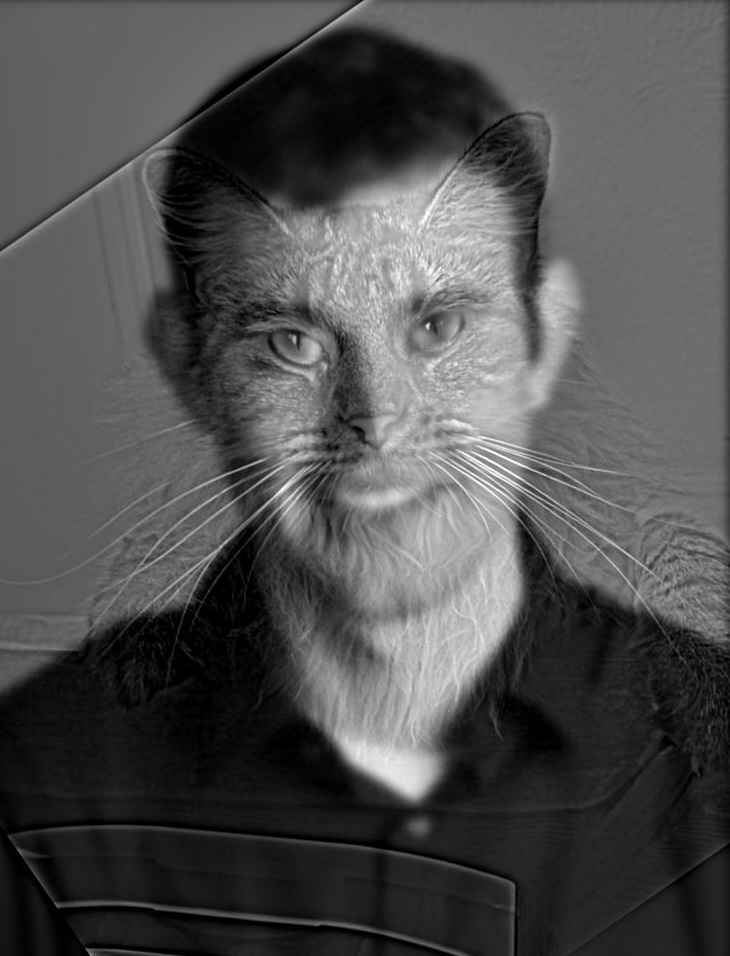
Curry and Fox

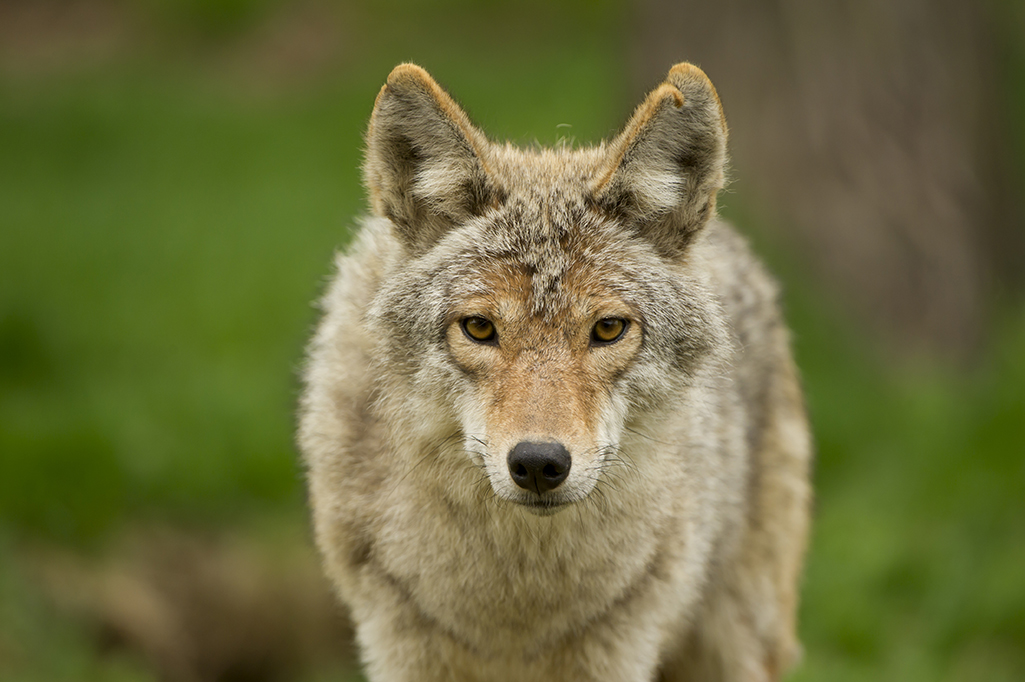
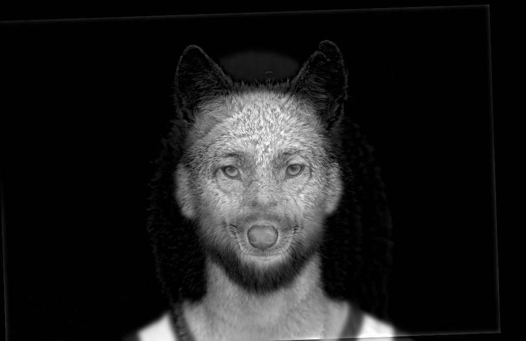
My Girlfriend Jessi and Panda (Fail Case) (Hopefully, she won't beat me up.)

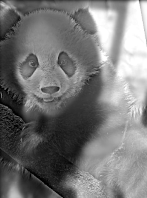
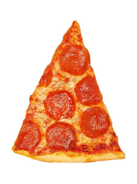
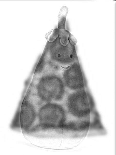
Pizza and Jellycat (Favorite)

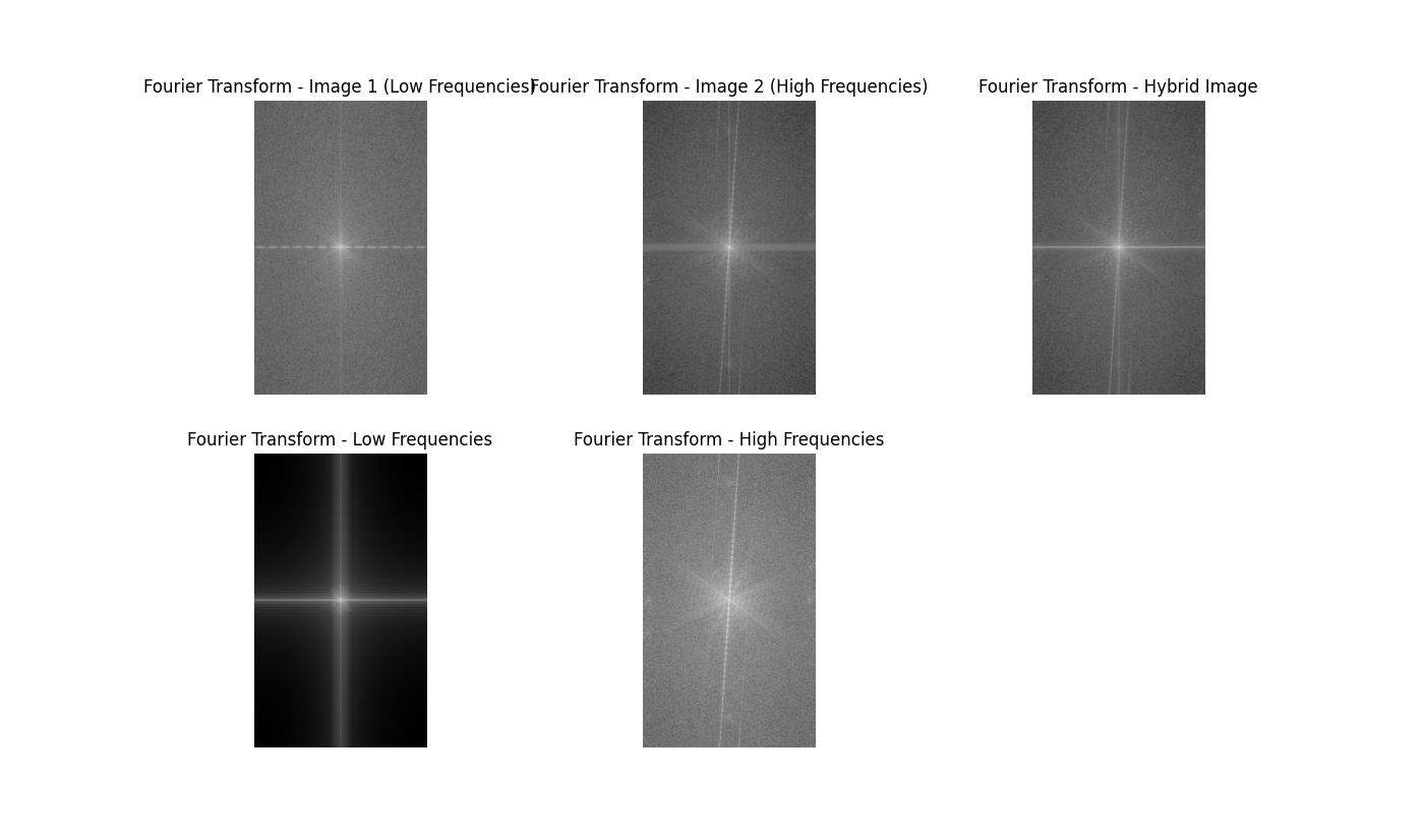
Frequency Analysis

Part 2.3: Gaussian and Laplacian Stacks

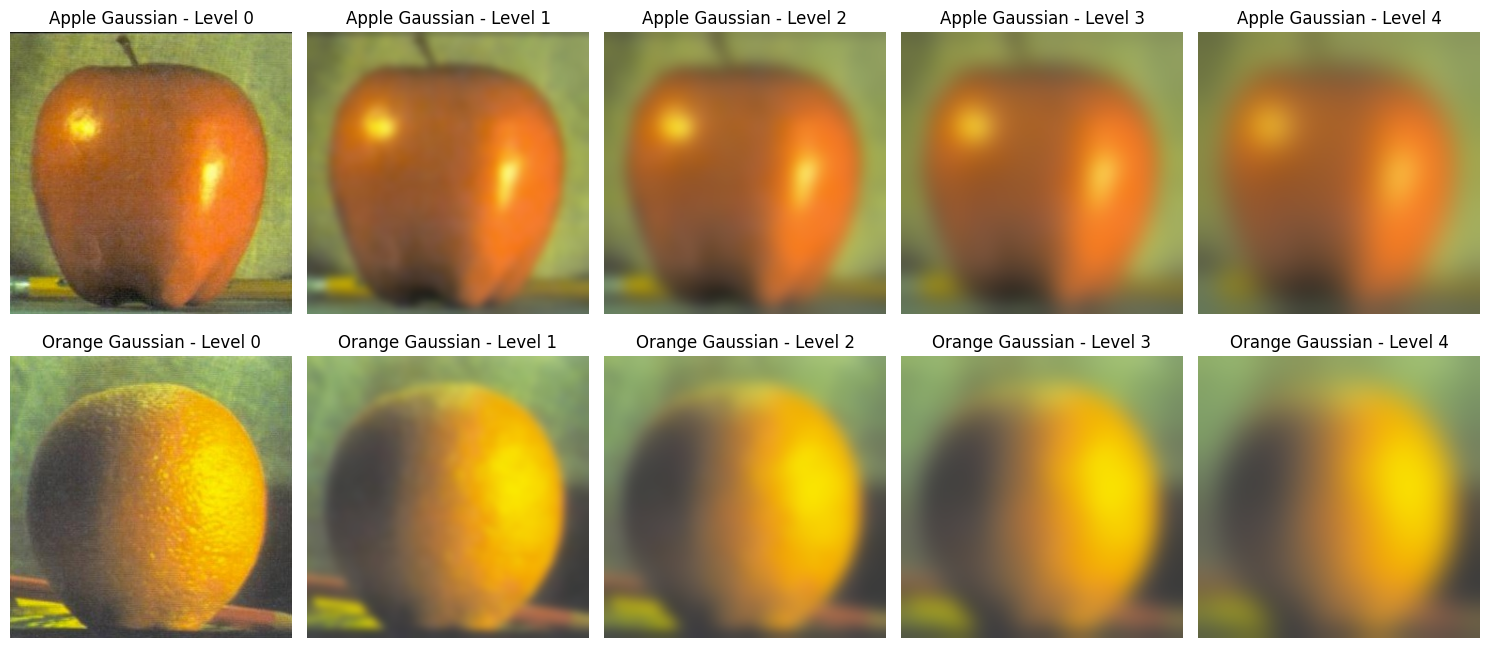
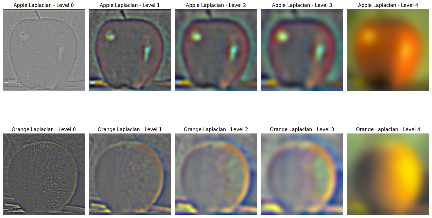
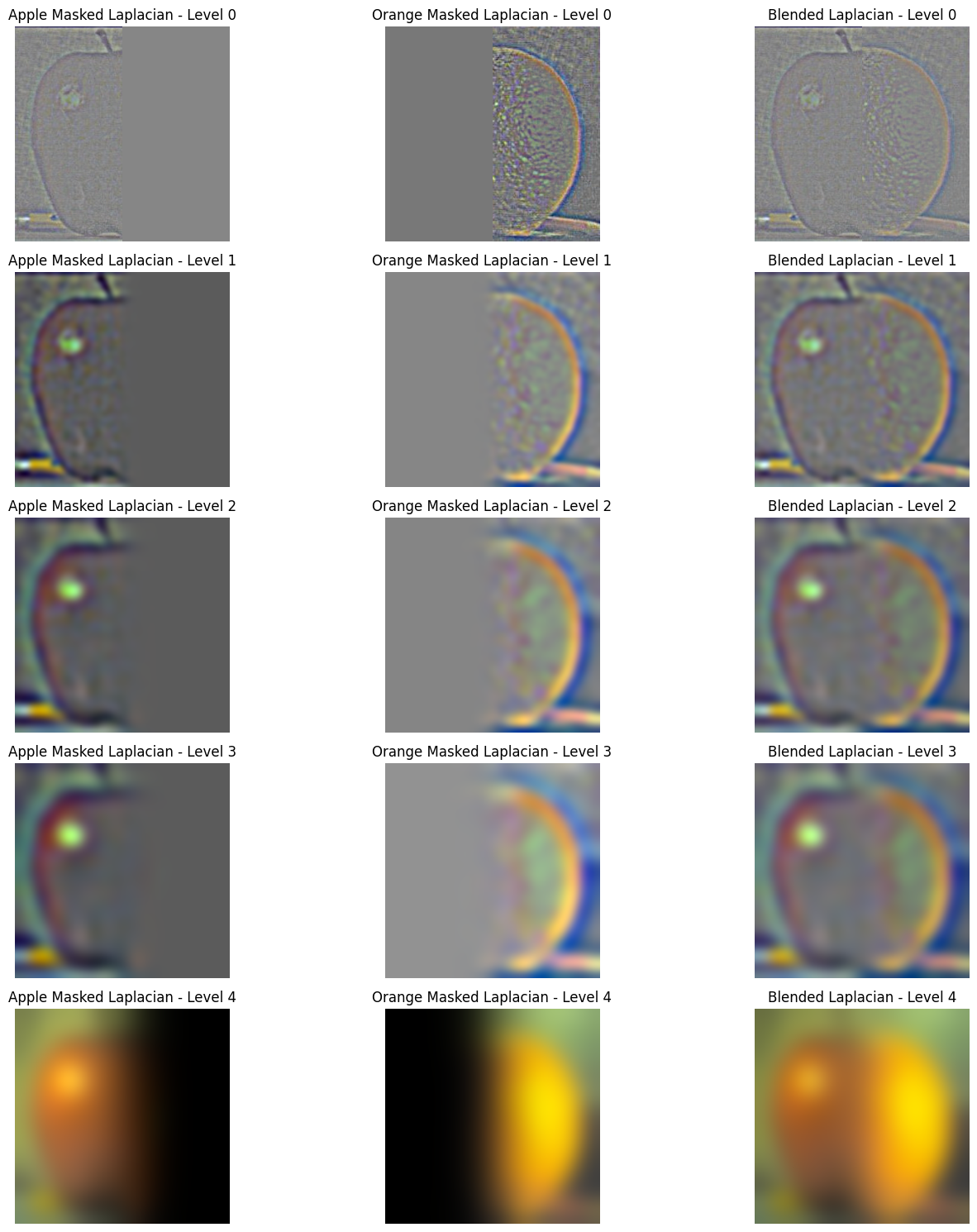
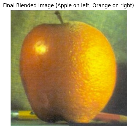
Part 2.4: Multiresolution Blending (a.k.a. the oraple!)

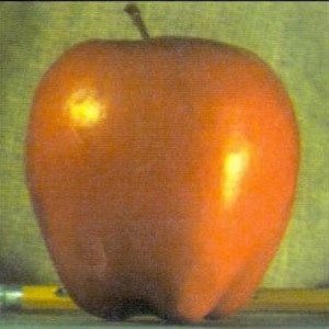
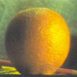
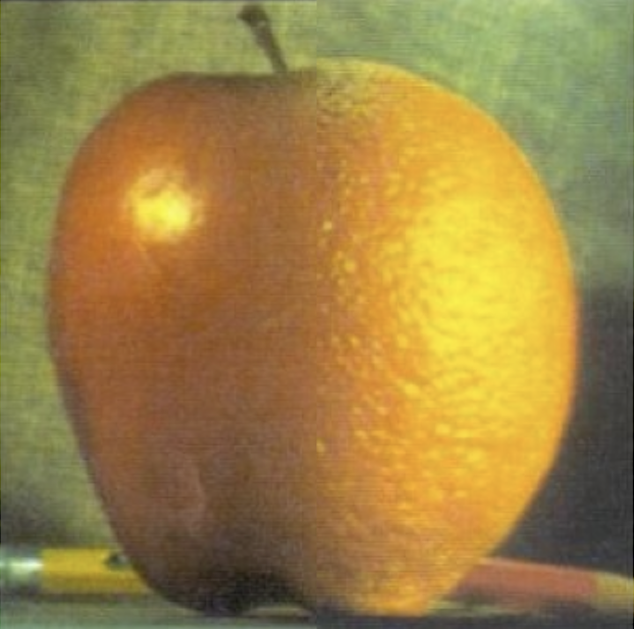
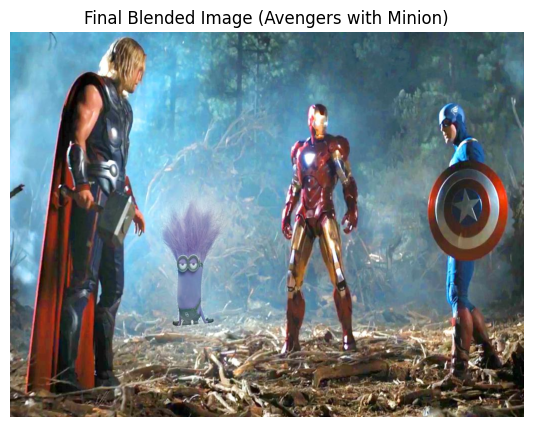
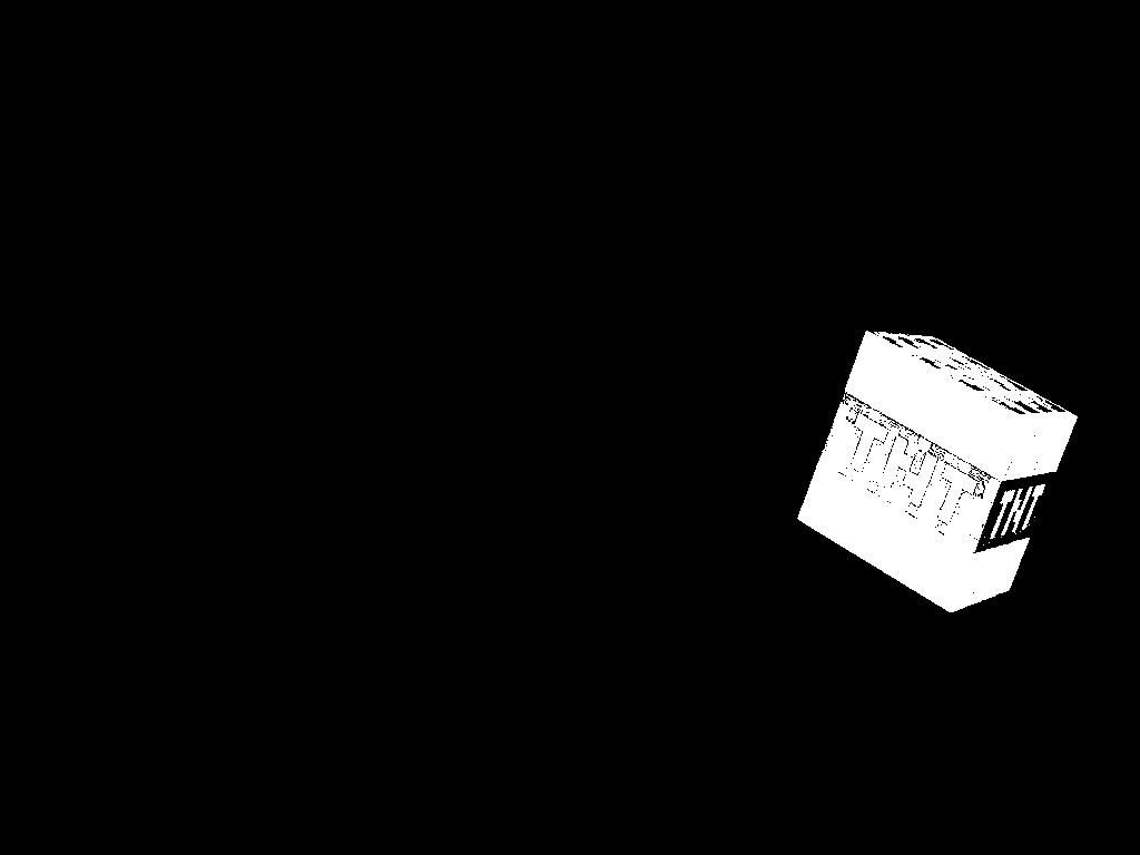
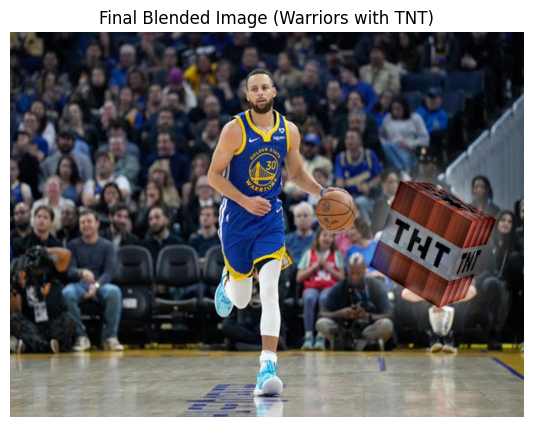
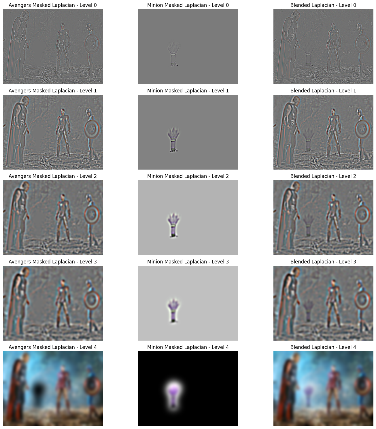
The avengers and minion is my favorite. Below are the Laplacian stacks for this blended image.

Takeaways: One of the most important things I learned from this project is how critical different frequency components are in shaping an image's appearance. Low-frequency components capture the overall structure and smooth transitions, while high-frequency components define sharp edges and fine details. Through tasks like hybrid images and multiresolution blending, I realized that manipulating these frequencies allows us to control which parts of an image dominate perception, depending on the viewing distance or how the image is processed. For example, high frequencies are key to enhancing sharpness and edges, but too much can introduce noise. On the other hand, low frequencies give an image its general shape but can obscure important details if overused. This project deepened my understanding of how balancing these frequencies is essential to achieving both clarity and visual appeal in image processing.